Alien-XGBoost
view release on metacpan or search on metacpan
xgboost/doc/model.md view on Meta::CPAN
```math
\hat{y}_i^{(0)} &= 0\\
\hat{y}_i^{(1)} &= f_1(x_i) = \hat{y}_i^{(0)} + f_1(x_i)\\
\hat{y}_i^{(2)} &= f_1(x_i) + f_2(x_i)= \hat{y}_i^{(1)} + f_2(x_i)\\
&\dots\\
\hat{y}_i^{(t)} &= \sum_{k=1}^t f_k(x_i)= \hat{y}_i^{(t-1)} + f_t(x_i)
```
It remains to ask, which tree do we want at each step? A natural thing is to add the one that optimizes our objective.
```math
\text{obj}^{(t)} & = \sum_{i=1}^n l(y_i, \hat{y}_i^{(t)}) + \sum_{i=1}^t\Omega(f_i) \\
& = \sum_{i=1}^n l(y_i, \hat{y}_i^{(t-1)} + f_t(x_i)) + \Omega(f_t) + constant
```
If we consider using MSE as our loss function, it becomes the following form.
```math
\text{obj}^{(t)} & = \sum_{i=1}^n (y_i - (\hat{y}_i^{(t-1)} + f_t(x_i)))^2 + \sum_{i=1}^t\Omega(f_i) \\
& = \sum_{i=1}^n [2(\hat{y}_i^{(t-1)} - y_i)f_t(x_i) + f_t(x_i)^2] + \Omega(f_t) + constant
```
The form of MSE is friendly, with a first order term (usually called the residual) and a quadratic term.
For other losses of interest (for example, logistic loss), it is not so easy to get such a nice form.
So in the general case, we take the Taylor expansion of the loss function up to the second order
```math
\text{obj}^{(t)} = \sum_{i=1}^n [l(y_i, \hat{y}_i^{(t-1)}) + g_i f_t(x_i) + \frac{1}{2} h_i f_t^2(x_i)] + \Omega(f_t) + constant
```
where the ``$g_i$`` and ``$h_i$`` are defined as
```math
g_i &= \partial_{\hat{y}_i^{(t-1)}} l(y_i, \hat{y}_i^{(t-1)})\\
h_i &= \partial_{\hat{y}_i^{(t-1)}}^2 l(y_i, \hat{y}_i^{(t-1)})
```
After we remove all the constants, the specific objective at step ``$t$`` becomes
```math
\sum_{i=1}^n [g_i f_t(x_i) + \frac{1}{2} h_i f_t^2(x_i)] + \Omega(f_t)
```
This becomes our optimization goal for the new tree. One important advantage of this definition is that
it only depends on ``$g_i$`` and ``$h_i$``. This is how xgboost can support custom loss functions.
We can optimize every loss function, including logistic regression and weighted logistic regression, using exactly
the same solver that takes ``$g_i$`` and ``$h_i$`` as input!
### Model Complexity
We have introduced the training step, but wait, there is one important thing, the ***regularization***!
We need to define the complexity of the tree ``$\Omega(f)$``. In order to do so, let us first refine the definition of the tree ``$ f(x) $`` as
```math
f_t(x) = w_{q(x)}, w \in R^T, q:R^d\rightarrow \{1,2,\cdots,T\} .
```
Here ``$ w $`` is the vector of scores on leaves, ``$ q $`` is a function assigning each data point to the corresponding leaf, and ``$ T $`` is the number of leaves.
In XGBoost, we define the complexity as
```math
\Omega(f) = \gamma T + \frac{1}{2}\lambda \sum_{j=1}^T w_j^2
```
Of course there is more than one way to define the complexity, but this specific one works well in practice. The regularization is one part most tree packages treat
less carefully, or simply ignore. This was because the traditional treatment of tree learning only emphasized improving impurity, while the complexity control was left to heuristics.
By defining it formally, we can get a better idea of what we are learning, and yes it works well in practice.
### The Structure Score
Here is the magical part of the derivation. After reformalizing the tree model, we can write the objective value with the ``$ t$``-th tree as:
```math
Obj^{(t)} &\approx \sum_{i=1}^n [g_i w_{q(x_i)} + \frac{1}{2} h_i w_{q(x_i)}^2] + \gamma T + \frac{1}{2}\lambda \sum_{j=1}^T w_j^2\\
&= \sum^T_{j=1} [(\sum_{i\in I_j} g_i) w_j + \frac{1}{2} (\sum_{i\in I_j} h_i + \lambda) w_j^2 ] + \gamma T
```
where ``$ I_j = \{i|q(x_i)=j\} $`` is the set of indices of data points assigned to the ``$ j $``-th leaf.
Notice that in the second line we have changed the index of the summation because all the data points on the same leaf get the same score.
We could further compress the expression by defining ``$ G_j = \sum_{i\in I_j} g_i $`` and ``$ H_j = \sum_{i\in I_j} h_i $``:
```math
\text{obj}^{(t)} = \sum^T_{j=1} [G_jw_j + \frac{1}{2} (H_j+\lambda) w_j^2] +\gamma T
```
In this equation ``$ w_j $`` are independent with respect to each other, the form ``$ G_jw_j+\frac{1}{2}(H_j+\lambda)w_j^2 $`` is quadratic and the best ``$ w_j $`` for a given structure ``$q(x)$`` and the best objective reduction we can get is:
```math
w_j^\ast = -\frac{G_j}{H_j+\lambda}\\
\text{obj}^\ast = -\frac{1}{2} \sum_{j=1}^T \frac{G_j^2}{H_j+\lambda} + \gamma T
```
The last equation measures ***how good*** a tree structure ``$q(x)$`` is.
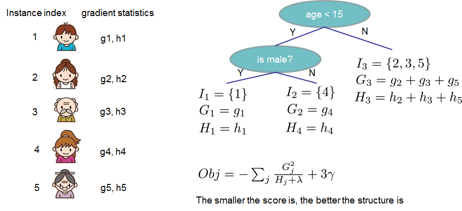
If all this sounds a bit complicated, let's take a look at the picture, and see how the scores can be calculated.
Basically, for a given tree structure, we push the statistics ``$g_i$`` and ``$h_i$`` to the leaves they belong to,
sum the statistics together, and use the formula to calculate how good the tree is.
This score is like the impurity measure in a decision tree, except that it also takes the model complexity into account.
### Learn the tree structure
Now that we have a way to measure how good a tree is, ideally we would enumerate all possible trees and pick the best one.
In practice this is intractable, so we will try to optimize one level of the tree at a time.
Specifically we try to split a leaf into two leaves, and the score it gains is
```math
Gain = \frac{1}{2} \left[\frac{G_L^2}{H_L+\lambda}+\frac{G_R^2}{H_R+\lambda}-\frac{(G_L+G_R)^2}{H_L+H_R+\lambda}\right] - \gamma
```
This formula can be decomposed as 1) the score on the new left leaf 2) the score on the new right leaf 3) The score on the original leaf 4) regularization on the additional leaf.
We can see an important fact here: if the gain is smaller than ``$\gamma$``, we would do better not to add that branch. This is exactly the ***pruning*** techniques in tree based
models! By using the principles of supervised learning, we can naturally come up with the reason these techniques work :)
For real valued data, we usually want to search for an optimal split. To efficiently do so, we place all the instances in sorted order, like the following picture.
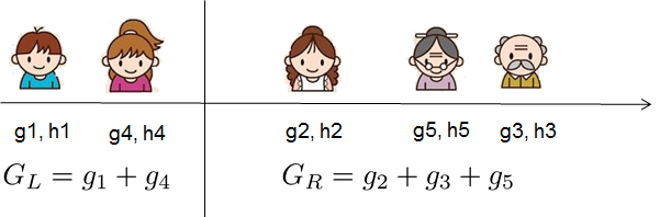
A left to right scan is sufficient to calculate the structure score of all possible split solutions, and we can find the best split efficiently.
Final words on XGBoost
----------------------
Now that you understand what boosted trees are, you may ask, where is the introduction on [XGBoost](https://github.com/dmlc/xgboost)?
XGBoost is exactly a tool motivated by the formal principle introduced in this tutorial!
More importantly, it is developed with both deep consideration in terms of ***systems optimization*** and ***principles in machine learning***.
The goal of this library is to push the extreme of the computation limits of machines to provide a ***scalable***, ***portable*** and ***accurate*** library.
Make sure you [try it out](https://github.com/dmlc/xgboost), and most importantly, contribute your piece of wisdom (code, examples, tutorials) to the community!
( run in 1.703 second using v1.01-cache-2.11-cpan-acf6aa7dc9e )