view release on metacpan or search on metacpan
xgboost/NEWS.md view on Meta::CPAN
  - has importance plot and tree plot functions.
  - accepts different learning rates for each boosting round.
  - allows model training continuation from previously saved model.
  - allows early stopping in CV.
  - allows feval to return a list of tuples.
  - allows eval_metric to handle additional format.
  - improved compatibility in sklearn module.
  - additional parameters added for sklearn wrapper.
  - added pip installation functionality.
  - supports more Pandas DataFrame dtypes.
  - added best_ntree_limit attribute, in addition to best_score and best_iteration.
* Java api is ready for use
* Added more test cases and continuous integration to make each build more robust.

## v0.4 (2015.05.11)

* Distributed version of xgboost that runs on YARN, scales to billions of examples
* Direct save/load data and model from/to S3 and HDFS
* Feature importance visualization in R module, by Michael Benesty
* Predict leaf index
* Poisson regression for counts data
xgboost/R-package/R/callbacks.R view on Meta::CPAN
#'
#' When a callback function has \code{finalize} parameter, its finalizer part will also be run after
#' the boosting is completed.
#'
#' WARNING: side-effects!!! Be aware that these callback functions access and modify things in
#' the environment from which they are called from, which is a fairly uncommon thing to do in R.
#'
#' To write a custom callback closure, make sure you first understand the main concepts about R envoronments.
#' Check either R documentation on \code{\link[base]{environment}} or the
#' \href{http://adv-r.had.co.nz/Environments.html}{Environments chapter} from the "Advanced R"
#' book by Hadley Wickham. Further, the best option is to read the code of some of the existing callbacks -
#' choose ones that do something similar to what you want to achieve. Also, you would need to get familiar
#' with the objects available inside of the \code{xgb.train} and \code{xgb.cv} internal environments.
#'
#' @seealso
#' \code{\link{cb.print.evaluation}},
#' \code{\link{cb.evaluation.log}},
#' \code{\link{cb.reset.parameters}},
#' \code{\link{cb.early.stop}},
#' \code{\link{cb.save.model}},
#' \code{\link{cb.cv.predict}},
xgboost/R-package/R/callbacks.R view on Meta::CPAN
#'        \code{metric_name='dtest-auc'} or \code{metric_name='dtest_auc'}.
#'        All dash '-' characters in metric names are considered equivalent to '_'.
#' @param verbose whether to print the early stopping information.
#'
#' @details
#' This callback function determines the condition for early stopping
#' by setting the \code{stop_condition = TRUE} flag in its calling frame.
#'
#' The following additional fields are assigned to the model's R object:
#' \itemize{
#' \item \code{best_score} the evaluation score at the best iteration
#' \item \code{best_iteration} at which boosting iteration the best score has occurred (1-based index)
#' \item \code{best_ntreelimit} to use with the \code{ntreelimit} parameter in \code{predict}.
#'      It differs from \code{best_iteration} in multiclass or random forest settings.
#' }
#'
#' The Same values are also stored as xgb-attributes:
#' \itemize{
#' \item \code{best_iteration} is stored as a 0-based iteration index (for interoperability of binary models)
#' \item \code{best_msg} message string is also stored.
#' }
#'
#' At least one data element is required in the evaluation watchlist for early stopping to work.
#'
#' Callback function expects the following values to be set in its calling frame:
#' \code{stop_condition},
#' \code{bst_evaluation},
#' \code{rank},
#' \code{bst} (or \code{bst_folds} and \code{basket}),
#' \code{iteration},
xgboost/R-package/R/callbacks.R view on Meta::CPAN
#' \code{num_parallel_tree}.
#'
#' @seealso
#' \code{\link{callbacks}},
#' \code{\link{xgb.attr}}
#'
#' @export
cb.early.stop <- function(stopping_rounds, maximize = FALSE,
                          metric_name = NULL, verbose = TRUE) {
  # state variables
  best_iteration <- -1
  best_ntreelimit <- -1
  best_score <- Inf
  best_msg <- NULL
  metric_idx <- 1

  init <- function(env) {
    if (length(env$bst_evaluation) == 0)
      stop("For early stopping, watchlist must have at least one element")

    eval_names <- gsub('-', '_', names(env$bst_evaluation))
    if (!is.null(metric_name)) {
      metric_idx <<- which(gsub('-', '_', metric_name) == eval_names)
      if (length(metric_idx) == 0)
xgboost/R-package/R/callbacks.R view on Meta::CPAN
    metric_name <<- eval_names[metric_idx]

    # maximize is usually NULL when not set in xgb.train and built-in metrics
    if (is.null(maximize))
      maximize <<- grepl('(_auc|_map|_ndcg)', metric_name)

    if (verbose && NVL(env$rank, 0) == 0)
      cat("Will train until ", metric_name, " hasn't improved in ",
          stopping_rounds, " rounds.\n\n", sep = '')

    best_iteration <<- 1
    if (maximize) best_score <<- -Inf

    env$stop_condition <- FALSE

    if (!is.null(env$bst)) {
      if (!inherits(env$bst, 'xgb.Booster'))
        stop("'bst' in the parent frame must be an 'xgb.Booster'")
      if (!is.null(best_score <- xgb.attr(env$bst$handle, 'best_score'))) {
        best_score <<- as.numeric(best_score)
        best_iteration <<- as.numeric(xgb.attr(env$bst$handle, 'best_iteration')) + 1
        best_msg <<- as.numeric(xgb.attr(env$bst$handle, 'best_msg'))
      } else {
        xgb.attributes(env$bst$handle) <- list(best_iteration = best_iteration - 1,
                                               best_score = best_score)
      }
    } else if (is.null(env$bst_folds) || is.null(env$basket)) {
      stop("Parent frame has neither 'bst' nor ('bst_folds' and 'basket')")
    }
  }

  finalizer <- function(env) {
    if (!is.null(env$bst)) {
      attr_best_score = as.numeric(xgb.attr(env$bst$handle, 'best_score'))
      if (best_score != attr_best_score)
        stop("Inconsistent 'best_score' values between the closure state: ", best_score,
             " and the xgb.attr: ", attr_best_score)
      env$bst$best_iteration = best_iteration
      env$bst$best_ntreelimit = best_ntreelimit
      env$bst$best_score = best_score
    } else {
      env$basket$best_iteration <- best_iteration
      env$basket$best_ntreelimit <- best_ntreelimit
    }
  }

  callback <- function(env = parent.frame(), finalize = FALSE) {
    if (best_iteration < 0)
      init(env)

    if (finalize)
      return(finalizer(env))

    i <- env$iteration
    score = env$bst_evaluation[metric_idx]

    if (( maximize && score > best_score) ||
        (!maximize && score < best_score)) {

      best_msg <<- format.eval.string(i, env$bst_evaluation, env$bst_evaluation_err)
      best_score <<- score
      best_iteration <<- i
      best_ntreelimit <<- best_iteration * env$num_parallel_tree
      # save the property to attributes, so they will occur in checkpoint
      if (!is.null(env$bst)) {
        xgb.attributes(env$bst) <- list(
          best_iteration = best_iteration - 1, # convert to 0-based index
          best_score = best_score,
          best_msg = best_msg,
          best_ntreelimit = best_ntreelimit)
      }
    } else if (i - best_iteration >= stopping_rounds) {
      env$stop_condition <- TRUE
      env$end_iteration <- i
      if (verbose && NVL(env$rank, 0) == 0)
        cat("Stopping. Best iteration:\n", best_msg, "\n\n", sep = '')
    }
  }
  attr(callback, 'call') <- match.call()
  attr(callback, 'name') <- 'cb.early.stop'
  callback
}


#' Callback closure for saving a model file.
#'
xgboost/R-package/R/callbacks.R view on Meta::CPAN
      stop("'cb.cv.predict' callback requires 'basket' and 'bst_folds' lists in its calling frame")

    N <- nrow(env$data)
    pred <-
      if (env$num_class > 1) {
        matrix(NA_real_, N, env$num_class)
      } else {
        rep(NA_real_, N)
      }

    ntreelimit <- NVL(env$basket$best_ntreelimit,
                      env$end_iteration * env$num_parallel_tree)
    if (NVL(env$params[['booster']], '') == 'gblinear') {
      ntreelimit <- 0 # must be 0 for gblinear
    }
    for (fd in env$bst_folds) {
      pr <- predict(fd$bst, fd$watchlist[[2]], ntreelimit = ntreelimit, reshape = TRUE)
      if (is.matrix(pred)) {
        pred[fd$index,] <- pr
      } else {
        pred[fd$index] <- pr
xgboost/R-package/R/xgb.Booster.R view on Meta::CPAN
#'
#' @rdname predict.xgb.Booster
#' @export
predict.xgb.Booster <- function(object, newdata, missing = NA, outputmargin = FALSE, ntreelimit = NULL,
                                predleaf = FALSE, predcontrib = FALSE, reshape = FALSE, ...) {

  object <- xgb.Booster.complete(object, saveraw = FALSE)
  if (!inherits(newdata, "xgb.DMatrix"))
    newdata <- xgb.DMatrix(newdata, missing = missing)
  if (is.null(ntreelimit))
    ntreelimit <- NVL(object$best_ntreelimit, 0)
  if (NVL(object$params[['booster']], '') == 'gblinear')
    ntreelimit <- 0
  if (ntreelimit < 0)
    stop("ntreelimit cannot be negative")

  option <- 0L + 1L * as.logical(outputmargin) + 2L * as.logical(predleaf) + 4L * as.logical(predcontrib)

  ret <- .Call(XGBoosterPredict_R, object$handle, newdata, option[1], as.integer(ntreelimit))

  n_ret <- length(ret)
xgboost/R-package/R/xgb.cv.R view on Meta::CPAN
#'         capture parameters changed by the \code{\link{cb.reset.parameters}} callback.
#'   \item \code{callbacks} callback functions that were either automatically assigned or
#'         explicitely passed.
#'   \item \code{evaluation_log} evaluation history storead as a \code{data.table} with the
#'         first column corresponding to iteration number and the rest corresponding to the
#'         CV-based evaluation means and standard deviations for the training and test CV-sets.
#'         It is created by the \code{\link{cb.evaluation.log}} callback.
#'   \item \code{niter} number of boosting iterations.
#'   \item \code{folds} the list of CV folds' indices - either those passed through the \code{folds}
#'         parameter or randomly generated.
#'   \item \code{best_iteration} iteration number with the best evaluation metric value
#'         (only available with early stopping).
#'   \item \code{best_ntreelimit} the \code{ntreelimit} value corresponding to the best iteration,
#'         which could further be used in \code{predict} method
#'         (only available with early stopping).
#'   \item \code{pred} CV prediction values available when \code{prediction} is set.
#'         It is either vector or matrix (see \code{\link{cb.cv.predict}}).
#'   \item \code{models} a liost of the CV folds' models. It is only available with the explicit
#'         setting of the \code{cb.cv.predict(save_models = TRUE)} callback.
#' }
#'
#' @examples
#' data(agaricus.train, package='xgboost')
xgboost/R-package/R/xgb.cv.R view on Meta::CPAN
#' Print xgb.cv result
#'
#' Prints formatted results of \code{xgb.cv}.
#'
#' @param x an \code{xgb.cv.synchronous} object
#' @param verbose whether to print detailed data
#' @param ... passed to \code{data.table.print}
#'
#' @details
#' When not verbose, it would only print the evaluation results,
#' including the best iteration (when available).
#'
#' @examples
#' data(agaricus.train, package='xgboost')
#' train <- agaricus.train
#' cv <- xgb.cv(data = train$data, label = train$label, nfold = 5, max_depth = 2,
#'                eta = 1, nthread = 2, nrounds = 2, objective = "binary:logistic")
#' print(cv)
#' print(cv, verbose=TRUE)
#'
#' @rdname print.xgb.cv
xgboost/R-package/R/xgb.cv.R view on Meta::CPAN
                 sep = ' = ', collapse = ', '), '\n', sep = '')
    }
    if (!is.null(x$callbacks) && length(x$callbacks) > 0) {
      cat('callbacks:\n')
      lapply(callback.calls(x$callbacks), function(x) {
        cat('  ')
        print(x)
      })
    }

    for (n in c('niter', 'best_iteration', 'best_ntreelimit')) {
      if (is.null(x[[n]]))
        next
      cat(n, ': ', x[[n]], '\n', sep = '')
    }

    if (!is.null(x$pred)) {
      cat('pred:\n')
      str(x$pred)
    }
  }

  if (verbose)
    cat('evaluation_log:\n')
  print(x$evaluation_log, row.names = FALSE, ...)

  if (!is.null(x$best_iteration)) {
    cat('Best iteration:\n')
    print(x$evaluation_log[x$best_iteration], row.names = FALSE, ...)
  }
  invisible(x)
}
xgboost/R-package/R/xgb.train.R view on Meta::CPAN
#'   \item \code{raw} a cached memory dump of the xgboost model saved as R's \code{raw} type.
#'   \item \code{niter} number of boosting iterations.
#'   \item \code{evaluation_log} evaluation history storead as a \code{data.table} with the
#'         first column corresponding to iteration number and the rest corresponding to evaluation
#'         metrics' values. It is created by the \code{\link{cb.evaluation.log}} callback.
#'   \item \code{call} a function call.
#'   \item \code{params} parameters that were passed to the xgboost library. Note that it does not
#'         capture parameters changed by the \code{\link{cb.reset.parameters}} callback.
#'   \item \code{callbacks} callback functions that were either automatically assigned or
#'         explicitely passed.
#'   \item \code{best_iteration} iteration number with the best evaluation metric value
#'         (only available with early stopping).
#'   \item \code{best_ntreelimit} the \code{ntreelimit} value corresponding to the best iteration,
#'         which could further be used in \code{predict} method
#'         (only available with early stopping).
#'   \item \code{best_score} the best evaluation metric value during early stopping.
#'         (only available with early stopping).
#'   \item \code{feature_names} names of the training dataset features
#'         (only when comun names were defined in training data).
#' }
#'
#' @seealso
#' \code{\link{callbacks}},
#' \code{\link{predict.xgb.Booster}},
#' \code{\link{xgb.cv}}
#'
xgboost/R-package/demo/caret_wrapper.R view on Meta::CPAN
require(xgboost)
require(data.table)
require(vcd)
require(e1071)

# Load Arthritis dataset in memory.
data(Arthritis)
# Create a copy of the dataset with data.table package (data.table is 100% compliant with R dataframe but its syntax is a lot more consistent and its performance are really good).
df <- data.table(Arthritis, keep.rownames = F)

# Let's add some new categorical features to see if it helps. Of course these feature are highly correlated to the Age feature. Usually it's not a good thing in ML, but Tree algorithms (including boosted trees) are able to select the best features, e...
# For the first feature we create groups of age by rounding the real age. Note that we transform it to factor (categorical data) so the algorithm treat them as independant values.
df[,AgeDiscret:= as.factor(round(Age/10,0))]

# Here is an even stronger simplification of the real age with an arbitrary split at 30 years old. I choose this value based on nothing. We will see later if simplifying the information based on arbitrary values is a good strategy (I am sure you alre...
df[,AgeCat:= as.factor(ifelse(Age > 30, "Old", "Young"))]

# We remove ID as there is nothing to learn from this feature (it will just add some noise as the dataset is small).
df[,ID:=NULL]

#-------------Basic Training using XGBoost in caret Library-----------------
xgboost/R-package/demo/create_sparse_matrix.R view on Meta::CPAN
df <- data.table(Arthritis, keep.rownames = F)

# Let's have a look to the data.table
cat("Print the dataset\n")
print(df)

# 2 columns have factor type, one has ordinal type (ordinal variable is a categorical variable with values wich can be ordered, here: None > Some > Marked).
cat("Structure of the dataset\n")
str(df)

# Let's add some new categorical features to see if it helps. Of course these feature are highly correlated to the Age feature. Usually it's not a good thing in ML, but Tree algorithms (including boosted trees) are able to select the best features, e...

# For the first feature we create groups of age by rounding the real age. Note that we transform it to factor (categorical data) so the algorithm treat them as independant values.
df[,AgeDiscret:= as.factor(round(Age/10,0))]

# Here is an even stronger simplification of the real age with an arbitrary split at 30 years old. I choose this value based on nothing. We will see later if simplifying the information based on arbitrary values is a good strategy (I am sure you alre...
df[,AgeCat:= as.factor(ifelse(Age > 30, "Old", "Young"))]

# We remove ID as there is nothing to learn from this feature (it will just add some noise as the dataset is small).
df[,ID:=NULL]
xgboost/R-package/demo/create_sparse_matrix.R view on Meta::CPAN
# Pearson correlation between Age and illness disappearing is 35

print(chisq.test(df$AgeDiscret, df$Y))
# Our first simplification of Age gives a Pearson correlation of 8.

print(chisq.test(df$AgeCat, df$Y))
# The perfectly random split I did between young and old at 30 years old have a low correlation of 2. It's a result we may expect as may be in my mind > 30 years is being old (I am 32 and starting feeling old, this may explain that), but  for the ill...

# As you can see, in general destroying information by simplifying it won't improve your model. Chi2 just demonstrates that. But in more complex cases, creating a new feature based on existing one which makes link with the outcome more obvious may he...
# However it's almost always worse when you add some arbitrary rules.
# Moreover, you can notice that even if we have added some not useful new features highly correlated with other features, the boosting tree algorithm have been able to choose the best one, which in this case is the Age. Linear model may not be that s...
xgboost/R-package/man/callbacks.Rd view on Meta::CPAN
When a callback function has \code{finalize} parameter, its finalizer part will also be run after
the boosting is completed.

WARNING: side-effects!!! Be aware that these callback functions access and modify things in
the environment from which they are called from, which is a fairly uncommon thing to do in R.

To write a custom callback closure, make sure you first understand the main concepts about R envoronments.
Check either R documentation on \code{\link[base]{environment}} or the
\href{http://adv-r.had.co.nz/Environments.html}{Environments chapter} from the "Advanced R"
book by Hadley Wickham. Further, the best option is to read the code of some of the existing callbacks -
choose ones that do something similar to what you want to achieve. Also, you would need to get familiar
with the objects available inside of the \code{xgb.train} and \code{xgb.cv} internal environments.
}
\seealso{
\code{\link{cb.print.evaluation}},
\code{\link{cb.evaluation.log}},
\code{\link{cb.reset.parameters}},
\code{\link{cb.early.stop}},
\code{\link{cb.save.model}},
\code{\link{cb.cv.predict}},
xgboost/R-package/man/cb.early.stop.Rd view on Meta::CPAN
}
\description{
Callback closure to activate the early stopping.
}
\details{
This callback function determines the condition for early stopping
by setting the \code{stop_condition = TRUE} flag in its calling frame.

The following additional fields are assigned to the model's R object:
\itemize{
\item \code{best_score} the evaluation score at the best iteration
\item \code{best_iteration} at which boosting iteration the best score has occurred (1-based index)
\item \code{best_ntreelimit} to use with the \code{ntreelimit} parameter in \code{predict}.
     It differs from \code{best_iteration} in multiclass or random forest settings.
}

The Same values are also stored as xgb-attributes:
\itemize{
\item \code{best_iteration} is stored as a 0-based iteration index (for interoperability of binary models)
\item \code{best_msg} message string is also stored.
}

At least one data element is required in the evaluation watchlist for early stopping to work.

Callback function expects the following values to be set in its calling frame:
\code{stop_condition},
\code{bst_evaluation},
\code{rank},
\code{bst} (or \code{bst_folds} and \code{basket}),
\code{iteration},
xgboost/R-package/man/print.xgb.cv.Rd view on Meta::CPAN
\item{verbose}{whether to print detailed data}

\item{...}{passed to \code{data.table.print}}
}
\description{
Prints formatted results of \code{xgb.cv}.
}
\details{
When not verbose, it would only print the evaluation results,
including the best iteration (when available).
}
\examples{
data(agaricus.train, package='xgboost')
train <- agaricus.train
cv <- xgb.cv(data = train$data, label = train$label, nfold = 5, max_depth = 2,
               eta = 1, nthread = 2, nrounds = 2, objective = "binary:logistic")
print(cv)
print(cv, verbose=TRUE)

}
xgboost/R-package/man/xgb.cv.Rd view on Meta::CPAN
        capture parameters changed by the \code{\link{cb.reset.parameters}} callback.
  \item \code{callbacks} callback functions that were either automatically assigned or
        explicitely passed.
  \item \code{evaluation_log} evaluation history storead as a \code{data.table} with the
        first column corresponding to iteration number and the rest corresponding to the
        CV-based evaluation means and standard deviations for the training and test CV-sets.
        It is created by the \code{\link{cb.evaluation.log}} callback.
  \item \code{niter} number of boosting iterations.
  \item \code{folds} the list of CV folds' indices - either those passed through the \code{folds}
        parameter or randomly generated.
  \item \code{best_iteration} iteration number with the best evaluation metric value
        (only available with early stopping).
  \item \code{best_ntreelimit} the \code{ntreelimit} value corresponding to the best iteration,
        which could further be used in \code{predict} method
        (only available with early stopping).
  \item \code{pred} CV prediction values available when \code{prediction} is set.
        It is either vector or matrix (see \code{\link{cb.cv.predict}}).
  \item \code{models} a liost of the CV folds' models. It is only available with the explicit
        setting of the \code{cb.cv.predict(save_models = TRUE)} callback.
}
}
\description{
The cross validation function of xgboost
xgboost/R-package/man/xgb.train.Rd view on Meta::CPAN
  \item \code{raw} a cached memory dump of the xgboost model saved as R's \code{raw} type.
  \item \code{niter} number of boosting iterations.
  \item \code{evaluation_log} evaluation history storead as a \code{data.table} with the
        first column corresponding to iteration number and the rest corresponding to evaluation
        metrics' values. It is created by the \code{\link{cb.evaluation.log}} callback.
  \item \code{call} a function call.
  \item \code{params} parameters that were passed to the xgboost library. Note that it does not
        capture parameters changed by the \code{\link{cb.reset.parameters}} callback.
  \item \code{callbacks} callback functions that were either automatically assigned or
        explicitely passed.
  \item \code{best_iteration} iteration number with the best evaluation metric value
        (only available with early stopping).
  \item \code{best_ntreelimit} the \code{ntreelimit} value corresponding to the best iteration,
        which could further be used in \code{predict} method
        (only available with early stopping).
  \item \code{best_score} the best evaluation metric value during early stopping.
        (only available with early stopping).
  \item \code{feature_names} names of the training dataset features
        (only when comun names were defined in training data).
}
}
\description{
\code{xgb.train} is an advanced interface for training an xgboost model.
The \code{xgboost} function is a simpler wrapper for \code{xgb.train}.
}
\details{
xgboost/R-package/tests/testthat/test_callbacks.R view on Meta::CPAN
  for (f in files) if (file.exists(f)) file.remove(f)
})

test_that("early stopping xgb.train works", {
  set.seed(11)
  expect_output(
    bst <- xgb.train(param, dtrain, nrounds = 20, watchlist, eta = 0.3,
                     early_stopping_rounds = 3, maximize = FALSE)
  , "Stopping. Best iteration")
  expect_false(is.null(bst$best_iteration))
  expect_lt(bst$best_iteration, 19)
  expect_equal(bst$best_iteration, bst$best_ntreelimit)

  pred <- predict(bst, dtest)
  expect_equal(length(pred), 1611)
  err_pred <- err(ltest, pred)
  err_log <- bst$evaluation_log[bst$best_iteration, test_error]
  expect_equal(err_log, err_pred, tolerance = 5e-6)

  set.seed(11)
  expect_silent(
    bst0 <- xgb.train(param, dtrain, nrounds = 20, watchlist, eta = 0.3,
                      early_stopping_rounds = 3, maximize = FALSE, verbose = 0)
  )
  expect_equal(bst$evaluation_log, bst0$evaluation_log)
})

test_that("early stopping using a specific metric works", {
  set.seed(11)
  expect_output(
    bst <- xgb.train(param, dtrain, nrounds = 20, watchlist, eta = 0.6,
                     eval_metric="logloss", eval_metric="auc",
                     callbacks = list(cb.early.stop(stopping_rounds = 3, maximize = FALSE,
                                                    metric_name = 'test_logloss')))
  , "Stopping. Best iteration")
  expect_false(is.null(bst$best_iteration))
  expect_lt(bst$best_iteration, 19)
  expect_equal(bst$best_iteration, bst$best_ntreelimit)

  pred <- predict(bst, dtest, ntreelimit = bst$best_ntreelimit)
  expect_equal(length(pred), 1611)
  logloss_pred <- sum(-ltest * log(pred) - (1 - ltest) * log(1 - pred)) / length(ltest)
  logloss_log <- bst$evaluation_log[bst$best_iteration, test_logloss]
  expect_equal(logloss_log, logloss_pred, tolerance = 5e-6)
})

test_that("early stopping xgb.cv works", {
  set.seed(11)
  expect_output(
    cv <- xgb.cv(param, dtrain, nfold = 5, eta = 0.3, nrounds = 20,
                 early_stopping_rounds = 3, maximize = FALSE)
  , "Stopping. Best iteration")
  expect_false(is.null(cv$best_iteration))
  expect_lt(cv$best_iteration, 19)
  expect_equal(cv$best_iteration, cv$best_ntreelimit)
  # the best error is min error:
  expect_true(cv$evaluation_log[, test_error_mean[cv$best_iteration] == min(test_error_mean)])
})

test_that("prediction in xgb.cv works", {
  set.seed(11)
  nrounds = 4
  cv <- xgb.cv(param, dtrain, nfold = 5, eta = 0.5, nrounds = nrounds, prediction = TRUE, verbose = 0)
  expect_false(is.null(cv$evaluation_log))
  expect_false(is.null(cv$pred))
  expect_length(cv$pred, nrow(train$data))
  err_pred <- mean( sapply(cv$folds, function(f) mean(err(ltrain[f], cv$pred[f]))) )
xgboost/R-package/tests/testthat/test_callbacks.R view on Meta::CPAN
  expect_length(cv$pred, nrow(train$data))
})

test_that("prediction in early-stopping xgb.cv works", {
  set.seed(1)
  expect_output(
    cv <- xgb.cv(param, dtrain, nfold = 5, eta = 0.1, nrounds = 20,
                 early_stopping_rounds = 5, maximize = FALSE, prediction = TRUE)
  , "Stopping. Best iteration")

  expect_false(is.null(cv$best_iteration))
  expect_lt(cv$best_iteration, 19)
  expect_false(is.null(cv$evaluation_log))
  expect_false(is.null(cv$pred))
  expect_length(cv$pred, nrow(train$data))

  err_pred <- mean( sapply(cv$folds, function(f) mean(err(ltrain[f], cv$pred[f]))) )
  err_log <- cv$evaluation_log[cv$best_iteration, test_error_mean]
  expect_equal(err_pred, err_log, tolerance = 1e-6)
  err_log_last <- cv$evaluation_log[cv$niter, test_error_mean]
  expect_gt(abs(err_pred - err_log_last), 1e-4)
})

test_that("prediction in xgb.cv for softprob works", {
  lb <- as.numeric(iris$Species) - 1
  set.seed(11)
  expect_warning(
    cv <- xgb.cv(data = as.matrix(iris[, -5]), label = lb, nfold = 4,
xgboost/R-package/vignettes/discoverYourData.Rmd view on Meta::CPAN
The method we are going to see is usually called [one-hot encoding](http://en.wikipedia.org/wiki/One-hot).

The first step is to load `Arthritis` dataset in memory and wrap it with `data.table` package.

```{r, results='hide'}
data(Arthritis)
df <- data.table(Arthritis, keep.rownames = F)
```

> `data.table` is 100% compliant with **R** `data.frame` but its syntax is more consistent and its performance for large dataset is [best in class](http://stackoverflow.com/questions/21435339/data-table-vs-dplyr-can-one-do-something-well-the-other-ca...

The first thing we want to do is to have a look to the first few lines of the `data.table`:

```{r}
head(df)
```

Now we will check the format of each column.

```{r}
xgboost/R-package/vignettes/discoverYourData.Rmd view on Meta::CPAN
Conclusion
----------

As you can see, in general *destroying information by simplifying it won't improve your model*. **Chi2** just demonstrates that.

But in more complex cases, creating a new feature based on existing one which makes link with the outcome more obvious may help the algorithm and improve the model.

The case studied here is not enough complex to show that. Check [Kaggle website](http://www.kaggle.com/) for some challenging datasets. However it's almost always worse when you add some arbitrary rules.

Moreover, you can notice that even if we have added some not useful new features highly correlated with other features, the boosting tree algorithm have been able to choose the best one, which in this case is the Age.

Linear model may not be that smart in this scenario.

Special Note: What about Random Forestsâ„¢?
-----------------------------------------

As you may know, [Random Forestsâ„¢](http://en.wikipedia.org/wiki/Random_forest) algorithm is cousin with boosting and both are part of the [ensemble learning](http://en.wikipedia.org/wiki/Ensemble_learning) family.

Both trains several decision trees for one dataset. The *main* difference is that in Random Forestsâ„¢, trees are independent and in boosting, the tree `N+1` focus its learning on the loss (<=> what has not been well modeled by the tree `N`).
xgboost/R-package/vignettes/xgboostPresentation.Rmd view on Meta::CPAN
**XGBoost** offers a way to group them in a `xgb.DMatrix`. You can even add other meta data in it. It will be useful for the most advanced features we will discover later.

```{r trainingDmatrix, message=F, warning=F}
dtrain <- xgb.DMatrix(data = train$data, label = train$label)
bstDMatrix <- xgboost(data = dtrain, max_depth = 2, eta = 1, nthread = 2, nrounds = 2, objective = "binary:logistic")
```

##### Verbose option

**XGBoost** has several features to help you to view how the learning progress internally. The purpose is to help you to set the best parameters, which is the key of your model quality.

One of the simplest way to see the training progress is to set the `verbose` option (see below for more advanced technics).

```{r trainingVerbose0, message=T, warning=F}
# verbose = 0, no message
bst <- xgboost(data = dtrain, max_depth = 2, eta = 1, nthread = 2, nrounds = 2, objective = "binary:logistic", verbose = 0)
```

```{r trainingVerbose1, message=T, warning=F}
# verbose = 1, print evaluation metric
xgboost/cub/CHANGE_LOG.TXT view on Meta::CPAN
1.0.2    08/23/2013
    - Corrections to code snippet examples for BlockLoad, BlockStore, and BlockDiscontinuity
    - Cleaned up unnecessary/missing header includes.  You can now safely #inlude a specific .cuh (instead of cub.cuh)
    - Bug/compilation fixes for BlockHistogram

//-----------------------------------------------------------------------------

1.0.1    08/08/2013
    - New collective interface idiom (specialize::construct::invoke).
    - Added best-in-class DeviceRadixSort.  Implements short-circuiting for homogenous digit passes.
    - Added best-in-class DeviceScan.  Implements single-pass "adaptive-lookback" strategy.
    - Significantly improved documentation (with example code snippets)
    - More extensive regression test suit for aggressively testing collective variants
    - Allow non-trially-constructed types (previously unions had prevented aliasing temporary storage of those types)
    - Improved support for Kepler SHFL (collective ops now use SHFL for types larger than 32b)
    - Better code generation for 64-bit addressing within BlockLoad/BlockStore
    - DeviceHistogram now supports histograms of arbitrary bins
    - Misc. fixes
      - Workarounds for SM10 codegen issues in uncommonly-used WarpScan/Reduce specializations
      - Updates to accommodate CUDA 5.5 dynamic parallelism
xgboost/cub/tune/tune_device_reduce.cu view on Meta::CPAN
 * LOSS OF USE, DATA, OR PROFITS; OR BUSINESS INTERRUPTION) HOWEVER CAUSED AND
 * ON ANY THEORY OF LIABILITY, WHETHER IN CONTRACT, STRICT LIABILITY, OR TORT
 * (INCLUDING NEGLIGENCE OR OTHERWISE) ARISING IN ANY WAY OUT OF THE USE OF THIS
 * SOFTWARE, EVEN IF ADVISED OF THE POSSIBILITY OF SUCH DAMAGE.
 *
 ******************************************************************************/

/******************************************************************************
 * Evaluates different tuning configurations of DeviceReduce.
 *
 * The best way to use this program:
 * (1) Find the best all-around single-block tune for a given arch.
 *     For example, 100 samples [1 ..512], 100 timing iterations per config per sample:
 *         ./bin/tune_device_reduce_sm200_nvvm_5.0_abi_i386 --i=100 --s=100 --n=512 --single --device=0
 * (2) Update the single tune in device_reduce.cuh
 * (3) Find the best all-around multi-block tune for a given arch.
 *     For example, 100 samples [single-block tile-size ..  50,331,648], 100 timing iterations per config per sample:
 *         ./bin/tune_device_reduce_sm200_nvvm_5.0_abi_i386 --i=100 --s=100 --device=0
 * (4) Update the multi-block tune in device_reduce.cuh
 *
 ******************************************************************************/

// Ensure printing of CUDA runtime errors to console
#define CUB_STDERR

#include <vector>
xgboost/cub/tune/tune_device_reduce.cu view on Meta::CPAN
    //---------------------------------------------------------------------

    /// Pairing of kernel function pointer and corresponding dispatch params
    template <typename KernelPtr>
    struct DispatchTuple
    {
        KernelPtr                           kernel_ptr;
        DeviceReduce::KernelDispachParams   params;

        float                               avg_throughput;
        float                               best_avg_throughput;
        OffsetT                              best_size;
        float                               hmean_speedup;


        DispatchTuple() :
            kernel_ptr(0),
            params(DeviceReduce::KernelDispachParams()),
            avg_throughput(0.0),
            best_avg_throughput(0.0),
            hmean_speedup(0.0),
            best_size(0)
        {}
    };

    /**
     * Comparison operator for DispatchTuple.avg_throughput
     */
    template <typename Tuple>
    static bool MinSpeedup(const Tuple &a, const Tuple &b)
    {
        float delta = a.hmean_speedup - b.hmean_speedup;

        return ((delta < 0.02) && (delta > -0.02)) ?
            (a.best_avg_throughput < b.best_avg_throughput) :       // Negligible average performance differences: defer to best performance
            (a.hmean_speedup < b.hmean_speedup);
    }


    /// Multi-block reduction kernel type and dispatch tuple type
    typedef void (*MultiBlockDeviceReduceKernelPtr)(T*, T*, OffsetT, GridEvenShare<OffsetT>, GridQueue<OffsetT>, ReductionOp);
    typedef DispatchTuple<MultiBlockDeviceReduceKernelPtr> MultiDispatchTuple;

    /// Single-block reduction kernel type and dispatch tuple type
xgboost/cub/tune/tune_device_reduce.cu view on Meta::CPAN
        }

        // Mooch
        CubDebugExit(cudaDeviceSynchronize());

        float avg_elapsed = elapsed_millis / g_timing_iterations;
        float avg_throughput = float(num_items) / avg_elapsed / 1000.0 / 1000.0;
        float avg_bandwidth = avg_throughput * sizeof(T);

        multi_dispatch.avg_throughput = CUB_MAX(avg_throughput, multi_dispatch.avg_throughput);
        if (avg_throughput > multi_dispatch.best_avg_throughput)
        {
            multi_dispatch.best_avg_throughput = avg_throughput;
            multi_dispatch.best_size = num_items;
        }

        single_dispatch.avg_throughput = CUB_MAX(avg_throughput, single_dispatch.avg_throughput);
        if (avg_throughput > single_dispatch.best_avg_throughput)
        {
            single_dispatch.best_avg_throughput = avg_throughput;
            single_dispatch.best_size = num_items;
        }

        if (g_verbose)
        {
            printf("\t%.2f GB/s, multi_dispatch( ", avg_bandwidth);
            multi_dispatch.params.Print();
            printf(" ), single_dispatch( ");
            single_dispatch.params.Print();
            printf(" )\n");
            fflush(stdout);
xgboost/cub/tune/tune_device_reduce.cu view on Meta::CPAN
            }
            if (g_verbose)
                printf("\n");
            else
                printf(", ");

            // Compute reference
            T h_reference = Reduce(h_in, reduction_op, num_items);

            // Run test on each multi-kernel configuration
            float best_avg_throughput = 0.0;
            for (int j = 0; j < multi_kernels.size(); ++j)
            {
                multi_kernels[j].avg_throughput = 0.0;

                TestConfiguration(multi_kernels[j], simple_single_tuple, d_in, d_out, &h_reference, num_items, reduction_op);

                best_avg_throughput = CUB_MAX(best_avg_throughput, multi_kernels[j].avg_throughput);
            }

            // Print best throughput for this problem size
            printf("Best: %.2fe9 items/s (%.2f GB/s)\n", best_avg_throughput, best_avg_throughput * sizeof(T));

            // Accumulate speedup (inverse for harmonic mean)
            for (int j = 0; j < multi_kernels.size(); ++j)
                multi_kernels[j].hmean_speedup += best_avg_throughput / multi_kernels[j].avg_throughput;
        }

        // Find max overall throughput and compute hmean speedups
        float overall_max_throughput = 0.0;
        for (int j = 0; j < multi_kernels.size(); ++j)
        {
            overall_max_throughput = CUB_MAX(overall_max_throughput, multi_kernels[j].best_avg_throughput);
            multi_kernels[j].hmean_speedup = float(g_samples) / multi_kernels[j].hmean_speedup;
        }

        // Sort by cumulative speedup
        sort(multi_kernels.begin(), multi_kernels.end(), MinSpeedup<MultiDispatchTuple>);

        // Print ranked multi configurations
        printf("\nRanked multi_kernels:\n");
        for (int j = 0; j < multi_kernels.size(); ++j)
        {
            printf("\t (%d) params( ", multi_kernels.size() - j);
            multi_kernels[j].params.Print();
            printf(" ) hmean speedup: %.3f, best throughput %.2f @ %d elements (%.2f GB/s, %.2f%%)\n",
                multi_kernels[j].hmean_speedup,
                multi_kernels[j].best_avg_throughput,
                (int) multi_kernels[j].best_size,
                multi_kernels[j].best_avg_throughput * sizeof(T),
                multi_kernels[j].best_avg_throughput / overall_max_throughput);
        }

        printf("\nMax multi-block throughput %.2f (%.2f GB/s)\n", overall_max_throughput, overall_max_throughput * sizeof(T));
    }


    /**
     * Evaluate single-block configurations
     */
    void TestSingle(
xgboost/cub/tune/tune_device_reduce.cu view on Meta::CPAN
            if (g_verbose)
                printf("\n");
            else
                printf(", ");

            // Compute reference
            T h_reference = Reduce(h_in, reduction_op, num_items);

            // Run test on each single-kernel configuration (pick first multi-config to use, which shouldn't be
            float best_avg_throughput = 0.0;
            for (int j = 0; j < single_kernels.size(); ++j)
            {
                single_kernels[j].avg_throughput = 0.0;

                TestConfiguration(multi_tuple, single_kernels[j], d_in, d_out, &h_reference, num_items, reduction_op);

                best_avg_throughput = CUB_MAX(best_avg_throughput, single_kernels[j].avg_throughput);
            }

            // Print best throughput for this problem size
            printf("Best: %.2fe9 items/s (%.2f GB/s)\n", best_avg_throughput, best_avg_throughput * sizeof(T));

            // Accumulate speedup (inverse for harmonic mean)
            for (int j = 0; j < single_kernels.size(); ++j)
                single_kernels[j].hmean_speedup += best_avg_throughput / single_kernels[j].avg_throughput;
        }

        // Find max overall throughput and compute hmean speedups
        float overall_max_throughput = 0.0;
        for (int j = 0; j < single_kernels.size(); ++j)
        {
            overall_max_throughput = CUB_MAX(overall_max_throughput, single_kernels[j].best_avg_throughput);
            single_kernels[j].hmean_speedup = float(g_samples) / single_kernels[j].hmean_speedup;
        }

        // Sort by cumulative speedup
        sort(single_kernels.begin(), single_kernels.end(), MinSpeedup<SingleDispatchTuple>);

        // Print ranked single configurations
        printf("\nRanked single_kernels:\n");
        for (int j = 0; j < single_kernels.size(); ++j)
        {
            printf("\t (%d) params( ", single_kernels.size() - j);
            single_kernels[j].params.Print();
            printf(" ) hmean speedup: %.3f, best throughput %.2f @ %d elements (%.2f GB/s, %.2f%%)\n",
                single_kernels[j].hmean_speedup,
                single_kernels[j].best_avg_throughput,
                (int) single_kernels[j].best_size,
                single_kernels[j].best_avg_throughput * sizeof(T),
                single_kernels[j].best_avg_throughput / overall_max_throughput);
        }

        printf("\nMax single-block throughput %.2f (%.2f GB/s)\n", overall_max_throughput, overall_max_throughput * sizeof(T));
    }

};


//---------------------------------------------------------------------
xgboost/demo/binary_classification/agaricus-lepiota.names view on Meta::CPAN
	Date: Mon, 17 Feb 1997 13:47:40 +0100
	From: Wlodzislaw Duch <duch@phys.uni.torun.pl>
	Organization: Dept. of Computer Methods, UMK

	I have attached a file containing logical rules for mushrooms.
	It should be helpful for other people since only in the last year I
	have seen about 10 papers analyzing this dataset and obtaining quite
	complex rules. We will try to contribute other results later.

	With best regards, Wlodek Duch
	________________________________________________________________

	Logical rules for the mushroom data sets.

	Logical rules given below seem to be the simplest possible for the
	mushroom dataset and therefore should be treated as benchmark results.

	Disjunctive rules for poisonous mushrooms, from most general
	to most specific:
xgboost/demo/guide-python/sklearn_examples.py view on Meta::CPAN
    print(mean_squared_error(actuals, predictions))

print("Parameter optimization")
y = boston['target']
X = boston['data']
xgb_model = xgb.XGBRegressor()
clf = GridSearchCV(xgb_model,
                   {'max_depth': [2,4,6],
                    'n_estimators': [50,100,200]}, verbose=1)
clf.fit(X,y)
print(clf.best_score_)
print(clf.best_params_)

# The sklearn API models are picklable
print("Pickling sklearn API models")
# must open in binary format to pickle
pickle.dump(clf, open("best_boston.pkl", "wb"))
clf2 = pickle.load(open("best_boston.pkl", "rb"))
print(np.allclose(clf.predict(X), clf2.predict(X)))

# Early-stopping

X = digits['data']
y = digits['target']
X_train, X_test, y_train, y_test = train_test_split(X, y, random_state=0)
clf = xgb.XGBClassifier()
clf.fit(X_train, y_train, early_stopping_rounds=10, eval_metric="auc",
        eval_set=[(X_test, y_test)])
xgboost/demo/guide-python/sklearn_parallel.py view on Meta::CPAN
    boston = load_boston()

    os.environ["OMP_NUM_THREADS"] = "2"  # or to whatever you want
    y = boston['target']
    X = boston['data']
    xgb_model = xgb.XGBRegressor()
    clf = GridSearchCV(xgb_model, {'max_depth': [2, 4, 6],
                                   'n_estimators': [50, 100, 200]}, verbose=1,
                       n_jobs=2)
    clf.fit(X, y)
    print(clf.best_score_)
    print(clf.best_params_)
xgboost/doc/Doxyfile view on Meta::CPAN
# enabled you may also need to install MathJax separately and configure the path
# to it using the MATHJAX_RELPATH option.
# The default value is: NO.
# This tag requires that the tag GENERATE_HTML is set to YES.

USE_MATHJAX            = NO

# When MathJax is enabled you can set the default output format to be used for
# the MathJax output. See the MathJax site (see:
# http://docs.mathjax.org/en/latest/output.html) for more details.
# Possible values are: HTML-CSS (which is slower, but has the best
# compatibility), NativeMML (i.e. MathML) and SVG.
# The default value is: HTML-CSS.
# This tag requires that the tag USE_MATHJAX is set to YES.

#MATHJAX_FORMAT         = HTML-CSS

# When MathJax is enabled you need to specify the location relative to the HTML
# output directory using the MATHJAX_RELPATH option. The destination directory
# should contain the MathJax.js script. For instance, if the mathjax directory
# is located at the same level as the HTML output directory, then
xgboost/doc/R-package/discoverYourData.md view on Meta::CPAN
The method we are going to see is usually called [one-hot encoding](http://en.wikipedia.org/wiki/One-hot).

The first step is to load `Arthritis` dataset in memory and wrap it with `data.table` package.


```r
data(Arthritis)
df <- data.table(Arthritis, keep.rownames = F)
```

> `data.table` is 100% compliant with **R** `data.frame` but its syntax is more consistent and its performance for large dataset is [best in class](http://stackoverflow.com/questions/21435339/data-table-vs-dplyr-can-one-do-something-well-the-other-ca...

The first thing we want to do is to have a look to the first lines of the `data.table`:


```r
head(df)
```

```
##    ID Treatment  Sex Age Improved
xgboost/doc/R-package/discoverYourData.md view on Meta::CPAN
Conclusion
----------

As you can see, in general *destroying information by simplifying it won't improve your model*. **Chi2** just demonstrates that.

But in more complex cases, creating a new feature based on existing one which makes link with the outcome more obvious may help the algorithm and improve the model.

The case studied here is not enough complex to show that. Check [Kaggle website](http://www.kaggle.com/) for some challenging datasets. However it's almost always worse when you add some arbitrary rules.

Moreover, you can notice that even if we have added some not useful new features highly correlated with other features, the boosting tree algorithm have been able to choose the best one, which in this case is the Age.

Linear models may not be that smart in this scenario.

Special Note: What about Random Forestsâ„¢?
-----------------------------------------

As you may know, [Random Forestsâ„¢](http://en.wikipedia.org/wiki/Random_forest) algorithm is cousin with boosting and both are part of the [ensemble learning](http://en.wikipedia.org/wiki/Ensemble_learning) family.

Both train several decision trees for one dataset. The *main* difference is that in Random Forestsâ„¢, trees are independent and in boosting, the tree `N+1` focus its learning on the loss (<=> what has not been well modeled by the tree `N`).
xgboost/doc/R-package/xgboostPresentation.md view on Meta::CPAN
bstDMatrix <- xgboost(data = dtrain, max.depth = 2, eta = 1, nthread = 2, nround = 2, objective = "binary:logistic")
```

```
## [0]	train-error:0.046522
## [1]	train-error:0.022263
```

##### Verbose option

**XGBoost** has several features to help you to view how the learning progress internally. The purpose is to help you to set the best parameters, which is the key of your model quality.

One of the simplest way to see the training progress is to set the `verbose` option (see below for more advanced technics).


```r
# verbose = 0, no message
bst <- xgboost(data = dtrain, max.depth = 2, eta = 1, nthread = 2, nround = 2, objective = "binary:logistic", verbose = 0)
```
xgboost/doc/_static/xgboost-theme/index.html view on Meta::CPAN
          Used in production by multiple companies.
        </p>
      </div>
      <div class="col-lg-4 col-sm-6">
        <h3><i class="fa fa-cloud"></i>Distributed on Cloud</h3>
        <p>Supports distributed training on multiple machines, including AWS,
          GCE, Azure, and Yarn clusters. Can be integrated with Flink, Spark and other cloud dataflow systems.</p>
      </div>
      <div class="col-lg-4 col-sm-6">
        <h3><i class="fa fa-rocket"></i> Performance</h3>
        <p>The well-optimized backend system for the best performance with limited resources.
          The distributed version solves problems beyond billions of examples with same code.
        </p>
      </div>
    </div>
  </div>
</div>
</div>
xgboost/doc/how_to/param_tuning.md view on Meta::CPAN
Understanding Bias-Variance Tradeoff
------------------------------------
If you take a machine learning or statistics course, this is likely to be one
of the most important concepts.
When we allow the model to get more complicated (e.g. more depth), the model
has better ability to fit the training data, resulting in a less biased model.
However, such complicated model requires more data to fit.

Most of parameters in xgboost are about bias variance tradeoff. The best model
should trade the model complexity with its predictive power carefully.
[Parameters Documentation](../parameter.md) will tell you whether each parameter
will make the model more conservative or not. This can be used to help you
turn the knob between complicated model and simple model.

Control Overfitting
-------------------
When you observe high training accuracy, but low tests accuracy, it is likely that you encounter overfitting problem.

There are in general two ways that you can control overfitting in xgboost
xgboost/doc/jvm/xgboost4j-intro.md view on Meta::CPAN
Programming languages and data processing/storage systems based on Java Virtual Machine (JVM) play the significant roles in the BigData ecosystem. [Hadoop](http://hadoop.apache.org/), [Spark](http://spark.apache.org/) and more recently introduced [Fl...

On the other side, the emerging demands of machine learning and deep learning
inspires many excellent machine learning libraries.
Many of these machine learning libraries(e.g. [XGBoost](https://github.com/dmlc/xgboost)/[MxNet](https://github.com/dmlc/mxnet))
requires new computation abstraction and native support (e.g. C++ for GPU computing).
They are also often [much more efficient](http://arxiv.org/abs/1603.02754).

The gap between the implementation fundamentals of the general data processing frameworks and the more specific machine learning libraries/systems prohibits the smooth connection between these two types of systems, thus brings unnecessary inconvenien...

We want best of both worlds, so we can use the data processing frameworks like Spark and Flink together with
the best distributed machine learning solutions.
To resolve the situation, we introduce the new-brewed [XGBoost4J](https://github.com/dmlc/xgboost/tree/master/jvm-packages),
<b>XGBoost</b> for <b>J</b>VM Platform. We aim to provide the clean Java/Scala APIs and the integration with the most popular data processing systems developed in JVM-based languages.

## Unix Philosophy in Machine Learning

XGBoost and XGBoost4J adopts Unix Philosophy.
XGBoost **does its best in one thing -- tree boosting** and is **being designed to work with other systems**.
We strongly believe that machine learning solution should not be restricted to certain language or certain platform.

Specifically, users will be able to use distributed XGBoost in both Spark and Flink, and possibly more frameworks in Future.
We have made the API in a portable way so it **can be easily ported to other Dataflow frameworks provided by the Cloud**.
XGBoost4J shares its core with other XGBoost libraries, which means data scientists can use R/python
read and visualize the model trained distributedly.
It also means that user can start with single machine version for exploration,
which already can handle hundreds of million examples.

## System Overview
xgboost/doc/jvm/xgboost4j-intro.md view on Meta::CPAN
xgboostModel.predict(testData.collect().iterator)

// distributed prediction
xgboostModel.predict(testData.map{x => x.vector})
```

## Road Map

It is the first release of XGBoost4J package, we are actively move forward for more charming features in the next release. You can watch our progress in [XGBoost4J Road Map](https://github.com/dmlc/xgboost/issues/935).

While we are trying our best to keep the minimum changes to the APIs, it is still subject to the incompatible changes.

## Further Readings

If you are interested in knowing more about XGBoost, you can find rich resources in

- [The github repository of XGBoost](https://github.com/dmlc/xgboost)
- [The comprehensive documentation site for XGBoostl](http://xgboost.readthedocs.org/en/latest/index.html)
- [An introduction to the gradient boosting model](http://xgboost.readthedocs.org/en/latest/model.html)
- [Tutorials for the R package](xgboost.readthedocs.org/en/latest/R-package/index.html)
- [Introduction of the Parameters](http://xgboost.readthedocs.org/en/latest/parameter.html)
xgboost/doc/jvm/xgboost4j_full_integration.md view on Meta::CPAN
val salesDF = spark.read.json("sales.json")
// call XGBoost API to train with the DataFrame-represented training set
val xgboostModel = XGBoost.trainWithDataFrame(
      salesDF, paramMap, numRound, nWorkers, useExternalMemory)
```

By integrating with DataFrame/Dataset, XGBoost4J-Spark not only enables users to call DataFrame/Dataset APIs directly but also make  DataFrame/Dataset-based Spark features available to XGBoost users, e.g. ML Package.

### Integration with ML Package

ML package of Spark provides a set of convenient tools for feature extraction/transformation/selection. Additionally, with the model selection tool in ML package, users can select the best model through an automatic parameter searching process which ...

#### Feature Extraction/Transformation/Selection

The following example shows a feature transformer which converts the string-typed storeType feature to the numeric storeTypeIndex. The transformed DataFrame is then fed to train XGBoost model.

```scala
import org.apache.spark.ml.feature.StringIndexer

// load sales records saved in json files
val salesDF = spark.read.json("sales.json")
xgboost/doc/model.md view on Meta::CPAN
For example, a common model is a *linear model*, where the prediction is given by ``$ \hat{y}_i = \sum_j \theta_j x_{ij} $``, a linear combination of weighted input features.
The prediction value can have different interpretations, depending on the task, i.e., regression or classification.
For example, it can be logistic transformed to get the probability of positive class in logistic regression, and it can also be used as a ranking score when we want to rank the outputs.

The ***parameters*** are the undetermined part that we need to learn from data. In linear regression problems, the parameters are the coefficients ``$ \theta $``.
Usually we will use ``$ \theta $`` to denote the parameters (there are many parameters in a model, our definition here is sloppy).

### Objective Function : Training Loss + Regularization

Based on different understandings of ``$ y_i $`` we can have different problems, such as regression, classification, ordering, etc.
We need to find a way to find the best parameters given the training data. In order to do so, we need to define a so-called ***objective function***,
to measure the performance of the model given a certain set of parameters.

A very important fact about objective functions is they ***must always*** contain two parts: training loss and regularization.

```math
Obj(\Theta) = L(\theta) + \Omega(\Theta)
```

where ``$ L $`` is the training loss function, and ``$ \Omega $`` is the regularization term. The training loss measures how *predictive* our model is on training data.
For example, a commonly used training loss is mean squared error.
xgboost/doc/model.md view on Meta::CPAN
```
Another commonly used loss function is logistic loss for logistic regression
```math
L(\theta) = \sum_i[ y_i\ln (1+e^{-\hat{y}_i}) + (1-y_i)\ln (1+e^{\hat{y}_i})]
```
The ***regularization term*** is what people usually forget to add. The regularization term controls the complexity of the model, which helps us to avoid overfitting.
This sounds a bit abstract, so let us consider the following problem in the following picture. You are asked to *fit* visually a step function given the input data points
on the upper left corner of the image.
Which solution among the three do you think is the best fit?
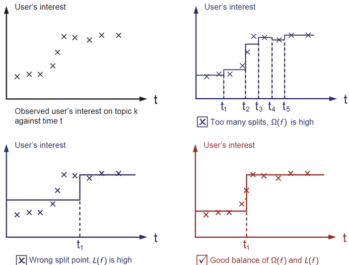
The correct answer is marked in red. Please consider if this visually seems a reasonable fit to you. The general principle is we want both a ***simple*** and ***predictive*** model.
The tradeoff between the two is also referred as bias-variance tradeoff in machine learning.
### Why introduce the general principle?
The elements introduced above form the basic elements of supervised learning, and they are naturally the building blocks of machine learning toolkits.
For example, you should be able to describe the differences and commonalities between boosted trees and random forests.
xgboost/doc/model.md view on Meta::CPAN
```
where ``$ I_j = \{i|q(x_i)=j\} $`` is the set of indices of data points assigned to the ``$ j $``-th leaf.
Notice that in the second line we have changed the index of the summation because all the data points on the same leaf get the same score.
We could further compress the expression by defining ``$ G_j = \sum_{i\in I_j} g_i $`` and ``$ H_j = \sum_{i\in I_j} h_i $``:
```math
\text{obj}^{(t)} = \sum^T_{j=1} [G_jw_j + \frac{1}{2} (H_j+\lambda) w_j^2] +\gamma T
```
In this equation ``$ w_j $`` are independent with respect to each other, the form ``$ G_jw_j+\frac{1}{2}(H_j+\lambda)w_j^2 $`` is quadratic and the best ``$ w_j $`` for a given structure ``$q(x)$`` and the best objective reduction we can get is:
```math
w_j^\ast = -\frac{G_j}{H_j+\lambda}\\
\text{obj}^\ast = -\frac{1}{2} \sum_{j=1}^T \frac{G_j^2}{H_j+\lambda} + \gamma T
```
The last equation measures ***how good*** a tree structure ``$q(x)$`` is.
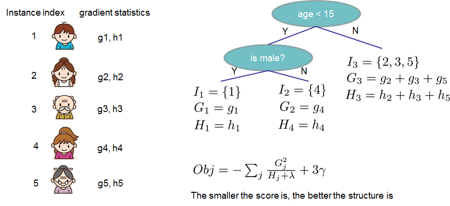
If all this sounds a bit complicated, let's take a look at the picture, and see how the scores can be calculated.
Basically, for a given tree structure, we push the statistics ``$g_i$`` and ``$h_i$`` to the leaves they belong to,
sum the statistics together, and use the formula to calculate how good the tree is.
This score is like the impurity measure in a decision tree, except that it also takes the model complexity into account.
### Learn the tree structure
Now that we have a way to measure how good a tree is, ideally we would enumerate all possible trees and pick the best one.
In practice this is intractable, so we will try to optimize one level of the tree at a time.
Specifically we try to split a leaf into two leaves, and the score it gains is
```math
Gain = \frac{1}{2} \left[\frac{G_L^2}{H_L+\lambda}+\frac{G_R^2}{H_R+\lambda}-\frac{(G_L+G_R)^2}{H_L+H_R+\lambda}\right] - \gamma
```
This formula can be decomposed as 1) the score on the new left leaf 2) the score on the new right leaf 3) The score on the original leaf 4) regularization on the additional leaf.
We can see an important fact here: if the gain is smaller than ``$\gamma$``, we would do better not to add that branch. This is exactly the ***pruning*** techniques in tree based
models! By using the principles of supervised learning, we can naturally come up with the reason these techniques work :)
For real valued data, we usually want to search for an optimal split. To efficiently do so, we place all the instances in sorted order, like the following picture.
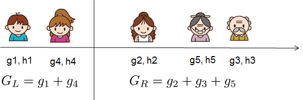
A left to right scan is sufficient to calculate the structure score of all possible split solutions, and we can find the best split efficiently.
Final words on XGBoost
----------------------
Now that you understand what boosted trees are, you may ask, where is the introduction on [XGBoost](https://github.com/dmlc/xgboost)?
XGBoost is exactly a tool motivated by the formal principle introduced in this tutorial!
More importantly, it is developed with both deep consideration in terms of ***systems optimization*** and ***principles in machine learning***.
The goal of this library is to push the extreme of the computation limits of machines to provide a ***scalable***, ***portable*** and ***accurate*** library.
Make sure you [try it out](https://github.com/dmlc/xgboost), and most importantly, contribute your piece of wisdom (code, examples, tutorials) to the community!
xgboost/doc/python/python_intro.md view on Meta::CPAN
Early Stopping
--------------
If you have a validation set, you can use early stopping to find the optimal number of boosting rounds.
Early stopping requires at least one set in `evals`. If there's more than one, it will use the last.

`train(..., evals=evals, early_stopping_rounds=10)`

The model will train until the validation score stops improving. Validation error needs to decrease at least every `early_stopping_rounds` to continue training.

If early stopping occurs, the model will have three additional fields: `bst.best_score`, `bst.best_iteration` and `bst.best_ntree_limit`. Note that `train()` will return a model from the last iteration, not the best one.

This works with both metrics to minimize (RMSE, log loss, etc.) and to maximize (MAP, NDCG, AUC). Note that if you specify more than one evaluation metric the last one in `param['eval_metric']` is used for early stopping.

Prediction
----------
A model that has been trained or loaded can perform predictions on data sets.
```python
# 7 entities, each contains 10 features
data = np.random.rand(7, 10)
dtest = xgb.DMatrix(data)
ypred = bst.predict(dtest)
```

If early stopping is enabled during training, you can get predictions from the best iteration with `bst.best_ntree_limit`:
```python
ypred = bst.predict(dtest,ntree_limit=bst.best_ntree_limit)
```

Plotting
--------

You can use plotting module to plot importance and output tree.

To plot importance, use ``plot_importance``. This function requires ``matplotlib`` to be installed.

```python
xgboost/doc/tutorials/aws_yarn.md view on Meta::CPAN
XGBoost is a portable framework, meaning the models in all platforms are ***exchangeable***.
This means we can load the trained model in python/R/Julia and take benefit of data science pipelines
in these languages to do model analysis and prediction.

For example, you can use [this IPython notebook](https://github.com/dmlc/xgboost/tree/master/demo/distributed-training/plot_model.ipynb)
to plot feature importance and visualize the learnt model.

Troubleshooting
----------------

If you encounter a problem, the best way might be to use the following command
to get logs of stdout and stderr of the containers and check what causes the problem.
```
yarn logs -applicationId yourAppId
```

Future Directions
-----------------
You have learned to use distributed XGBoost on YARN in this tutorial.
XGBoost is a portable and scalable framework for gradient boosting.
You can check out more examples and resources in the [resources page](https://github.com/dmlc/xgboost/blob/master/demo/README.md).

The project goal is to make the best scalable machine learning solution available to all platforms.
The API is designed to be able to portable, and the same code can also run on other platforms such as MPI and SGE.
XGBoost is actively evolving and we are working on even more exciting features
such as distributed xgboost python/R package. Checkout [RoadMap](https://github.com/dmlc/xgboost/issues/873) for
more details and you are more than welcomed to contribute to the project.